Decoding Volatility: From Log-Returns to the Yang-Zhang Estimator
· 3 min read

In the realm of quantitative finance, volatility is not just a measure of fear—it is the very fabric of risk and opportunity. To trade volatility is to trade the uncertainty of the future. However, how we measure this uncertainty has undergone a profound mathematical evolution, moving from simple static calculations to sophisticated dynamic estimators.
The Foundation: Logarithmic Returns
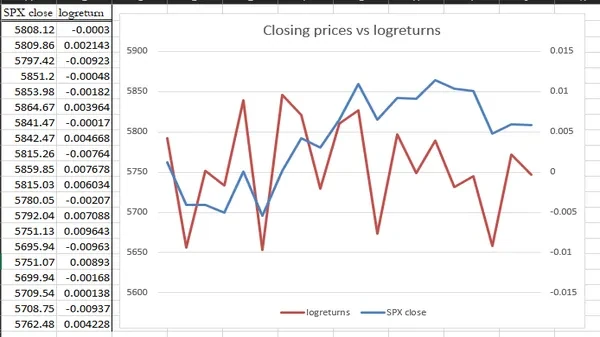
Before we can measure volatility, we must define how we calculate price changes. While retail traders often look at simple percentage returns, quantitative analysts rely exclusively on Logarithmic Returns (Log-Returns).
r_t = \ln\left(\frac{P_t}{P_{t-1}}\right) 1. **Time Additivity**: The log-return over two days is simply the sum of the log-returns of each day. 2. **Normalization**: Log-returns follow a more symmetric distribution, making them easier to model using the standard deviation. ## The Baseline: Standard Deviation (Close-to-Close) The most basic measure of volatility is the **Standard Deviation** ($\sigma$) of these log-returns over a specific window. While easy to calculate, it has a fatal flaw: it only looks at the closing prices, ignoring all the "chaos" that happens between the open and the close. ## The Evolution of Volatility Estimators To capture the true volatility of the market, mathematicians began looking at the entire price bar (Open, High, Low, Close). ### 1. The Parkinson Estimator (1980) Michael Parkinson was the first to realize that the **High-Low range** provides more information than just the close. * **Pros**: Much more efficient than simple standard deviation. * **Cons**: It assumes the market is a continuous process and ignores the "jumps" between yesterday's close and today's open. ### 2. The Garman-Klass Estimator (1980) Garman and Klass improved on Parkinson by including both the High-Low range and the Open-Close relationship. * **Insight**: It captures the "intra-day" volatility more accurately but still struggles with overnight price gaps. ### 3. The Rogers-Satchell Estimator (1991) Rogers and Satchell introduced an estimator that is independent of the market "Drift" (the general trend of the stock). This is critical for assets that are trending strongly in one direction. ## The Final Frontier: The Yang-Zhang Estimator (2000) The pinnacle of this mathematical journey is the **Yang-Zhang Estimator**. It is the first to successfully combine the best parts of the previous models while solving the most difficult problem in volatility measurement: **The Opening Jump**. Yang and Zhang realized that total volatility is the sum of three components: 1. **Overnight Volatility**: The gap between the previous close and the current open. 2. **Open-to-Close Volatility**: The movement within the trading day. 3. **The Weighted OHLC Range**: Integrating the Rogers-Satchell drift-independent logic. By merging these, Yang-Zhang provides a measure that is up to **14 times more efficient** than the simple close-to-close standard deviation. It is the comprehensive benchmark used by modern institutional quants to understand the true underlying risk of an asset. ## The Bottom Line Volatility is a multi-dimensional puzzle. From the early days of Parkinson to the modern sophistication of **Yang and Zhang**, our ability to quantify the unknown has reached a level of precision that was once thought impossible. At **Dashboard Options**, we utilize these advanced estimators to ensure that our volatility surfaces reflect the mathematical reality of the market, not just the noise. *Understanding the math is the first step to mastering the trade. Are you measuring the close, or are you measuring the reality?*